

Central question
Do machine-learning and hybrid models improve Bitcoin volatility forecasts beyond GARCH and simple benchmarks - and do any gains survive seed, rolling-window and untouched-test checks?
Project overview
This project builds a leakage-aware Bitcoin volatility forecasting pipeline using 4,239 daily BTC-USD returns from 2 January 2015 to 10 August 2026. The primary target is next-day squared return, with Parkinson variance used as a secondary robustness proxy.
The study compares historical variance, a 30-day rolling estimator, EWMA, sGARCH, XGBoost, LSTM, GRU and two GARCH-neural combinations. Model choice is made on the chronological validation period; the final test period is reserved for one unbiased performance assessment.
2 January 2015 - 10 August 2026
Selected GARCH-LSTM combination
Untouched 637-day test period
GARCH : LSTM, chosen on validation data
Evidence summary
A strong GARCH core with a small neural correction
The report separates model selection from final testing, then checks neural stability across random seeds and rolling windows before interpreting the 30-day risk path.01 · Data and volatility signature
Bitcoin returns were stationary, heavy-tailed and strongly clustered
The price level trended over time, while transformed returns provided the stationary series needed for volatility modelling.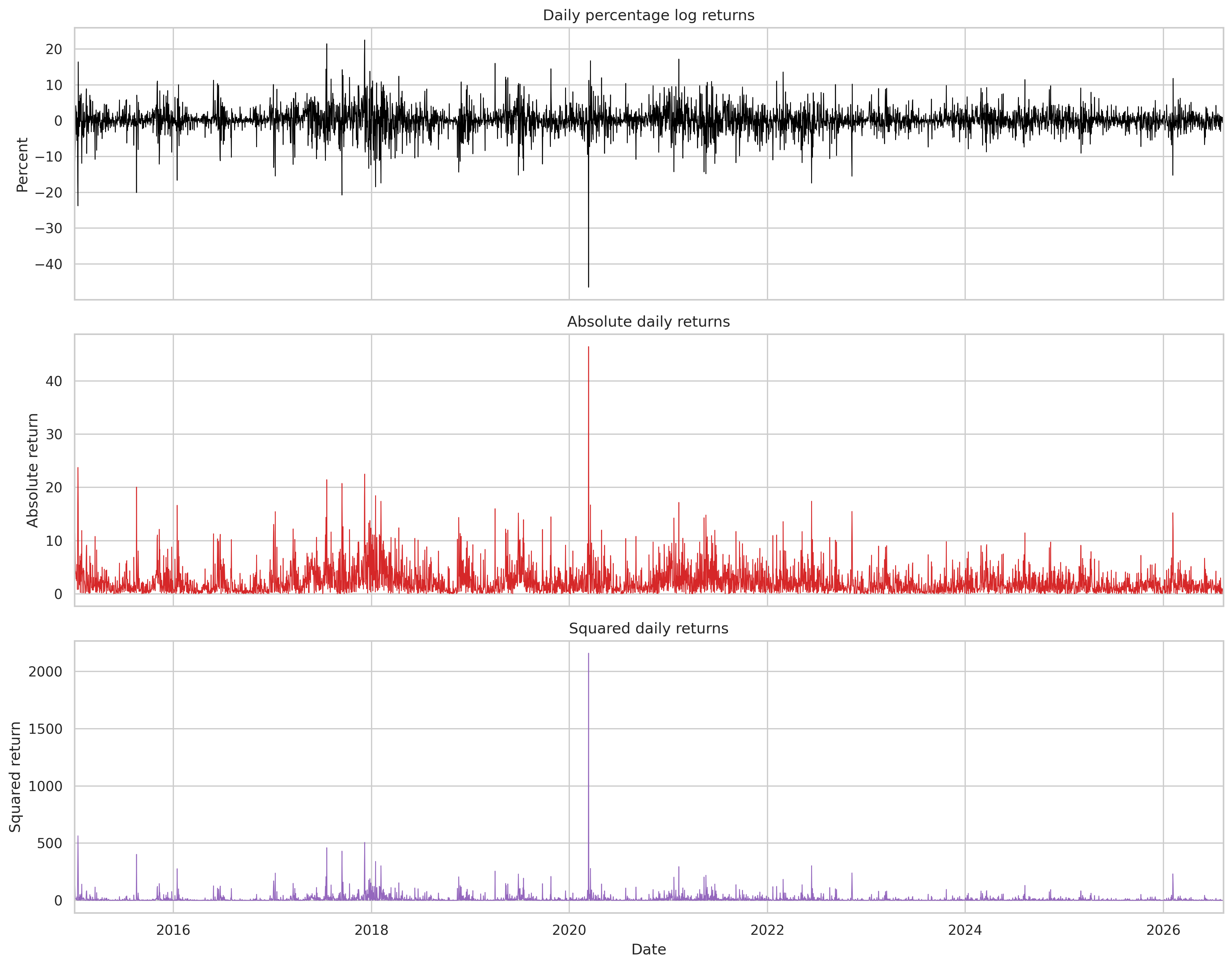
| Sample | Start | End | Observations |
|---|---|---|---|
| Training | 2 Jan 2015 | 15 Feb 2023 | 2,967 |
| Validation | 16 Feb 2023 | 11 Nov 2024 | 635 |
| Test | 12 Nov 2024 | 10 Aug 2026 | 637 |
What it showsThe analysis used 4,239 daily returns from January 2015 to August 2026. Returns had −0.74 skewness, 12.16 excess kurtosis and a −46.47% minimum on 12 March 2020. Absolute and squared returns formed visible high- and low-volatility regimes.
Why it mattersStrong squared-return autocorrelation and an ARCH-LM p-value below .001 establish time-varying conditional variance. A constant-variance model would miss the persistence visible after large shocks.
LimitationSquared return is an unbiased yet extremely noisy volatility proxy. One exceptional observation can dominate its scale, so QLIKE and a secondary Parkinson proxy are used alongside ordinary error measures.
02 · Econometric foundation
sGARCH captured the variance dynamics, with important boundary warnings
The mean and variance equations were selected separately, using training fit for ARMA and validation QLIKE for GARCH.| Candidate | QLIKE | RMSE | MAE | Correlation |
|---|---|---|---|---|
| sGARCH(1,1) · skewed t | 1.95326 | 13.944 | 8.456 | .144 |
| sGARCH(1,1) · Student t | 1.95329 | 13.943 | 8.449 | .144 |
| APARCH(1,1) · Student t | 1.96248 | 14.017 | 8.443 | .127 |
| GJR-GARCH(1,1) · Student t | 1.96370 | 14.025 | 8.459 | .128 |
| sGARCH(1,1) · normal | 1.97647 | 14.110 | 9.366 | .152 |
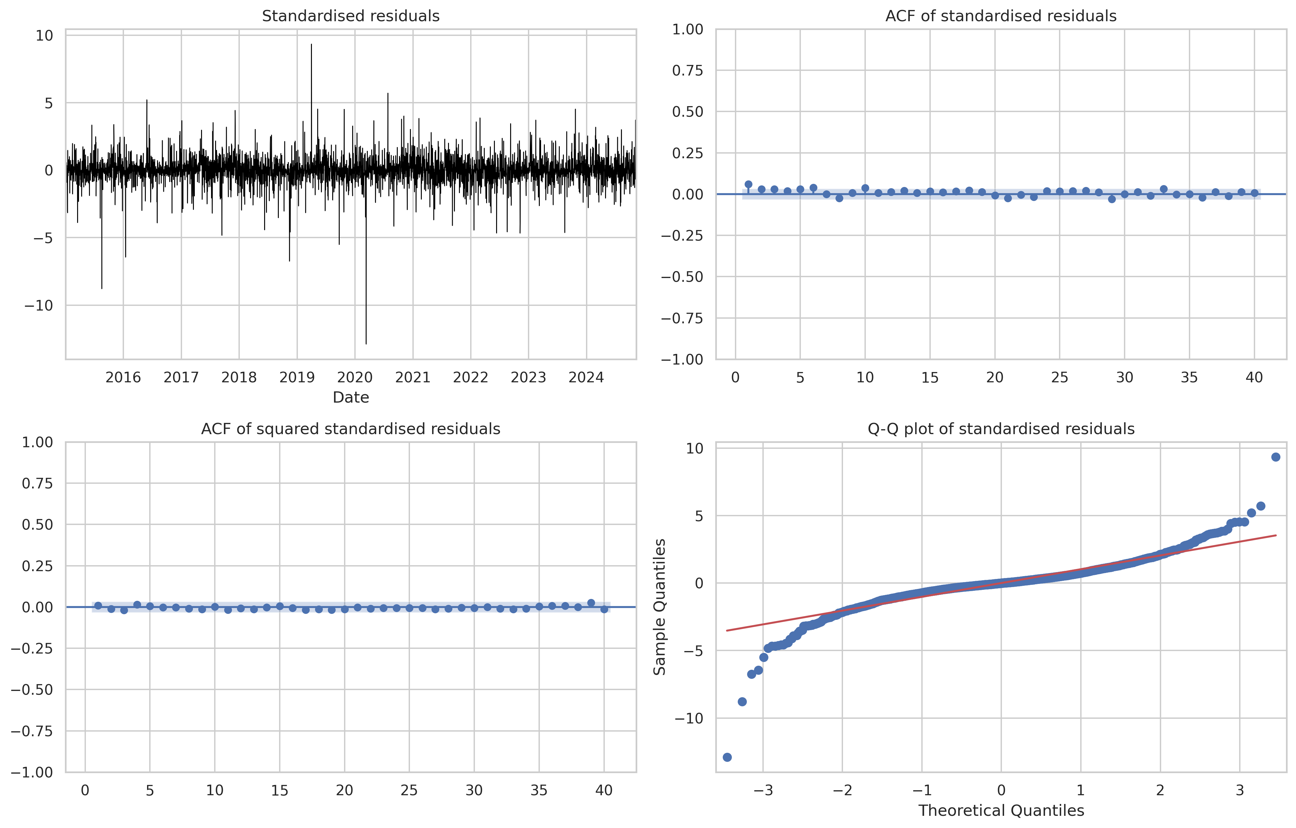
What it showsARMA(0,1) removed the remaining linear return dependence. The skewed-t sGARCH(1,1) achieved validation QLIKE 1.95326, only 0.00003 below the symmetric Student-t version. Its alpha and beta estimates summed to approximately one.
Why it mattersSquared standardised residuals showed no remaining autocorrelation and the post-fit ARCH-LM p-value was .997. The variance equation therefore captured the main volatility clustering pattern.
LimitationStandardised residuals retained some serial correlation and the Q-Q plot still showed extreme tails. The skew parameter was insignificant, while near-unit persistence makes long-run variance and half-life estimates unstable.
03 · Neural stability
Early stopping controlled a visible training-validation gap
LSTM and GRU results were repeated across five seeds and three rolling validation windows rather than relying on one favourable run.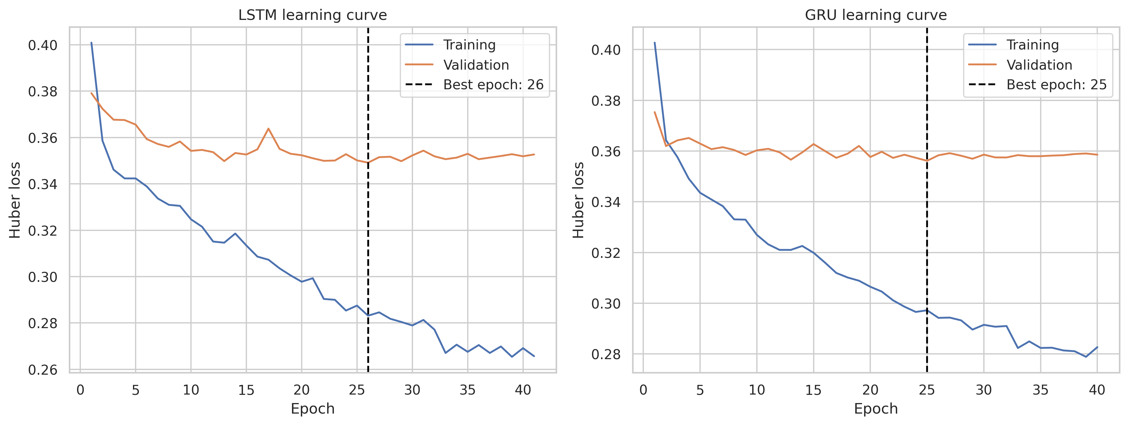
| Model | 5-seed validation | 5-seed test | Rolling mean | Rolling CV |
|---|---|---|---|---|
| Selected GARCH | - | - | 1.953 | 13.6% |
| GRU | 4.050 | 3.300 | 4.372 | 24.4% |
| LSTM | 4.123 | 3.313 | 4.766 | 23.9% |
| XGBoost | - | - | 4.667 | 9.6% |
What it showsTraining Huber loss continued falling after validation loss had flattened. Across five seeds, mean test QLIKE was 3.300 for GRU and 3.313 for LSTM. Across three rolling windows, mean QLIKE rose to 4.372 and 4.766 respectively, versus 1.953 for GARCH.
Why it mattersThe seed runs show that the neural ranking was not driven by one random initialisation. The rolling windows reveal that the standalone networks were less stable across market regimes than the econometric model.
LimitationThe apparent training-versus-test RMSE gap is influenced by a much more volatile early training era. Cross-period loss levels should not be interpreted as a conventional random-split overfitting ratio.
04 · Validation-led selection
The neural model helped most when it remained a small part of the forecast
Combination weights were chosen only on validation QLIKE, preserving the test period for final assessment.| Model | QLIKE | RMSE | MAE | Correlation |
|---|---|---|---|---|
| GARCH-LSTM · 82/18 | 1.94252 | 13.783 | 7.806 | .149 |
| GARCH-GRU · 85/15 | 1.94592 | 13.806 | 7.926 | .149 |
| Selected sGARCH | 1.95326 | 13.944 | 8.456 | .144 |
| EWMA | 2.00269 | 13.840 | 7.600 | .125 |
| 30-day rolling variance | 2.09800 | 13.945 | 7.486 | .100 |
| XGBoost | 4.49237 | 14.642 | 5.945 | .172 |
| GRU | 4.63837 | 14.501 | 6.022 | .132 |
| LSTM | 4.95199 | 14.520 | 5.923 | .129 |
What it showsAn 82% GARCH / 18% LSTM blend achieved the lowest validation QLIKE at 1.94252. The 85% GARCH / 15% GRU blend followed at 1.94592, while standalone GARCH scored 1.95326.
Why it mattersThe selected blend improved validation QLIKE by roughly 0.55% relative to GARCH. The small neural weight shows that the added value was a correction to the econometric forecast, not evidence that the network could replace it.
LimitationXGBoost, LSTM and GRU reported lower MAE while producing QLIKE above 4.49. Metric choice changes the apparent winner; QLIKE was prioritised for the positive, highly noisy variance target.
05 · Untouched test period
The selected hybrid retained its advantage without becoming a post-hoc winner
The 637-day test period was scored once after the GARCH-LSTM blend had been selected on validation data.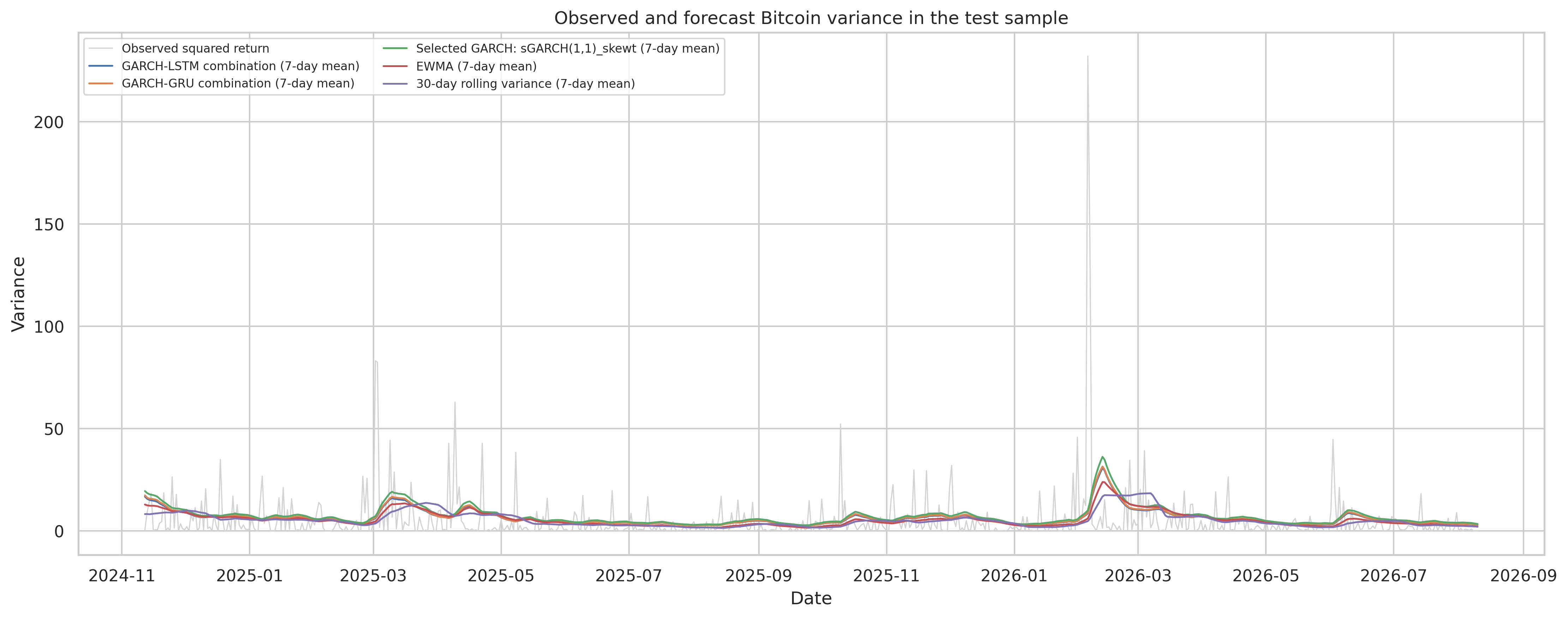
| Model | QLIKE | RMSE | MAE | Correlation |
|---|---|---|---|---|
| GARCH-GRU · post-test numeric low | 1.72974 | 13.565 | 6.562 | .206 |
| GARCH-LSTM · preselected | 1.73043 | 13.584 | 6.478 | .195 |
| Selected sGARCH | 1.76128 | 13.805 | 7.098 | .191 |
| EWMA | 1.76163 | 13.686 | 6.124 | .152 |
| 30-day rolling variance | 1.83824 | 13.875 | 6.050 | .102 |
| XGBoost | 3.43967 | 13.986 | 4.753 | .362 |
| GRU | 3.51443 | 13.745 | 4.734 | .341 |
| LSTM | 3.89424 | 14.053 | 4.783 | .146 |
What it showsGARCH-LSTM achieved test QLIKE 1.73043, RMSE 13.584 and MAE 6.478. GARCH-GRU was numerically lower at 1.72974, while its Diebold-Mariano comparison with the selected model had p = .870.
Why it mattersThe selected hybrid significantly reduced QLIKE loss relative to standalone GARCH (p = .0026). The same ordering held against Parkinson variance, where GARCH-LSTM scored 0.5402 versus 0.5629 for GARCH.
LimitationThe improvement over EWMA was not significant (p = .195). Forecast curves captured changing regimes yet still smoothed over isolated squared-return spikes, a common limitation when the target is extremely noisy.
06 · Calibration and forecast comparison
Statistical tests support a qualified, not absolute, winner
Calibration regressions and Diebold-Mariano tests distinguish numerical rankings from meaningful forecast differences.| Model | Intercept | Slope | Joint p-value | 5% decision |
|---|---|---|---|---|
| GARCH-LSTM | 1.095 | .665 | .178 | Do not reject |
| GARCH-GRU | .918 | .677 | .092 | Do not reject |
| EWMA | 2.153 | .559 | .201 | Do not reject |
| Selected sGARCH | 1.279 | .549 | < .001 | Reject |
| Comparator | DM statistic | p-value | Interpretation |
|---|---|---|---|
| GARCH-GRU | −0.164 | .870 | No significant difference |
| EWMA | 1.297 | .195 | No significant difference |
| Selected sGARCH | 3.027 | .0026 | Higher loss |
| LSTM | 3.333 | < .001 | Higher loss |
| XGBoost | 5.579 | < .001 | Higher loss |
| Historical variance | 9.589 | < .001 | Higher loss |
What it showsThe Mincer-Zarnowitz joint test did not reject intercept zero and slope one for GARCH-LSTM (p = .178), GARCH-GRU (p = .092) or EWMA (p = .201). Standalone GARCH was rejected (p < .001).
Why it mattersQLIKE differences versus GARCH, standalone neural models and historical variance were statistically meaningful. The selected model was not distinguishable from GARCH-GRU or EWMA at 5%.
LimitationFailure to reject ideal calibration does not prove it. Squared-return measurement noise and a finite test period reduce the power of forecast-comparison tests.
07 · Thirty-day scenario
The refitted GARCH model projected rising conditional risk
The future chart is a variance-model scenario, not a Bitcoin price forecast or a trading recommendation.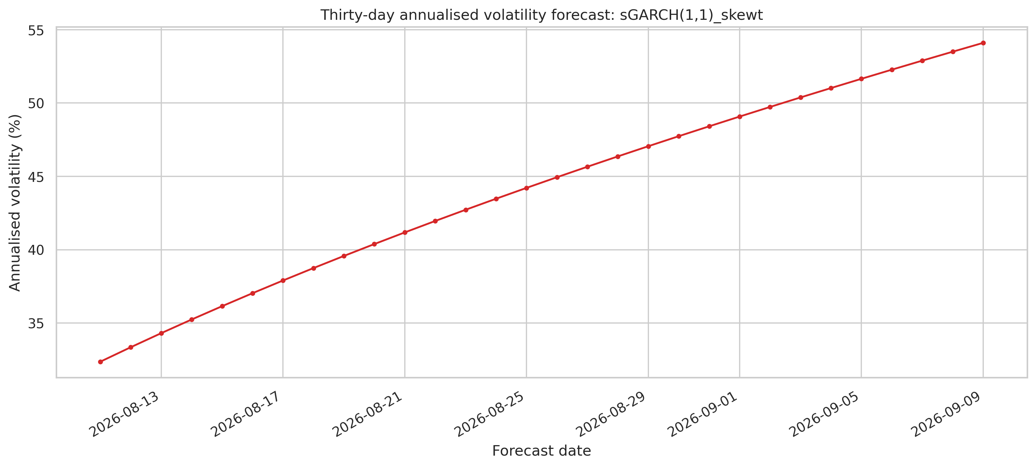
| Forecast date | Variance | Daily volatility | Annualised volatility |
|---|---|---|---|
| 11 Aug 2026 | 2.870 | 1.69% | 32.37% |
| 25 Aug 2026 | 5.356 | 2.31% | 44.21% |
| 9 Sep 2026 | 8.019 | 2.83% | 54.10% |
What it showsAnnualised conditional volatility rises from 32.4% on 11 August to 44.2% on 25 August and 54.1% on 9 September 2026. Daily conditional volatility rises from 1.69% to 2.83%.
Why it mattersThe path communicates the level and direction of model-implied uncertainty after the final observation. It is useful for risk scenarios, position limits and sensitivity analysis.
LimitationAlpha plus beta is approximately one, so shocks decay extremely slowly and the long-run variance is not stable. The rising curve is highly specification-sensitive and should not be treated as an investment signal.
Why a volatility model was required
Bitcoin prices were nonstationary, while daily returns were stationary under both ADF and KPSS evidence. Returns were heavy-tailed and negatively skewed: excess kurtosis was 12.16, the largest daily loss was −46.47%, and the Jarque-Bera test strongly rejected normality.
Raw returns showed limited serial dependence, while absolute and squared returns were strongly autocorrelated. The ARCH-LM test was also highly significant. Together, these results identify volatility clustering and justify modelling conditional variance rather than treating risk as constant through time.
- Training: 2,967 observations ending 15 February 2023.
- Validation: 635 observations from 16 February 2023 to 11 November 2024.
- Test: 637 observations from 12 November 2024 to 10 August 2026.
- All predictors were lagged or rolling features available before the forecast target.
Econometric foundation
ARMA(0,1) was selected for the conditional mean using the training-sample BIC. Its residual Ljung-Box p-values at lags 7, 14 and 30 were above 0.12, indicating that the short mean equation removed the remaining linear serial dependence adequately.
Among ARCH, sGARCH, GJR-GARCH, EGARCH and APARCH candidates, sGARCH(1,1) with skewed Student-t innovations achieved the lowest validation QLIKE at 1.95326. The Student-t alternative was virtually tied, and the skew parameter was not statistically significant, so the distributional distinction should not be overstated.
The selected variance model removed the remaining ARCH pattern: squared standardised-residual Ljung-Box p-values exceeded 0.86 and the 30-lag ARCH-LM p-value was 0.997. Some serial dependence remained in standardised residuals, while the Q-Q plot still showed extreme tails.
Machine learning and robustness checks
XGBoost, LSTM and GRU used lagged returns, absolute and squared returns, rolling moments, range-based volatility estimators, volume and cyclical calendar features. Standalone machine-learning models achieved lower MAE than GARCH, yet their QLIKE values were much worse. This distinction matters: MAE rewards smaller point errors, while QLIKE is more appropriate for noisy variance targets and penalises severely underestimated risk.
Repeated runs across five random seeds produced mean test QLIKE values of 3.300 for GRU and 3.313 for LSTM. Three rolling validation windows were less favourable: mean QLIKE was 1.953 for GARCH, compared with 4.372 for GRU, 4.667 for XGBoost and 4.766 for LSTM. The neural learning curves also showed widening training-validation gaps, making early stopping essential.
Selected model and untouched-test result
Validation weight searches selected an 82% GARCH / 18% LSTM combination with QLIKE 1.94252, narrowly ahead of the 85% GARCH / 15% GRU combination at 1.94592 and standalone GARCH at 1.95326. The modest neural weight is the substantive finding: machine learning added a small correction to a strong econometric core rather than replacing it.
On the untouched test period, the preselected GARCH-LSTM model achieved QLIKE 1.73043, RMSE 13.5836 and MAE 6.4778. GARCH-GRU posted a slightly lower test QLIKE of 1.72974, yet it was not selected after seeing the test data and the difference was not statistically significant (Diebold-Mariano p = 0.870).
Relative to GARCH-LSTM, QLIKE loss was significantly higher for standalone GARCH (p = 0.0026), LSTM, GRU, XGBoost, the 30-day rolling estimator and historical variance. The difference from EWMA was not significant (p = 0.195). A Mincer-Zarnowitz joint test did not reject ideal calibration for GARCH-LSTM (p = 0.178), although that result should not be read as proof of perfect calibration.
Thirty-day risk outlook and limitations
After refitting the selected sGARCH specification to the full sample, the model projected annualised volatility rising from 32.4% on 11 August 2026 to 54.1% on 9 September 2026. This is a conditional risk path rather than a Bitcoin price forecast.
The fitted GARCH coefficients sum to approximately one, indicating near-unit volatility persistence. That feature explains the slow decay of shocks and makes the long-horizon path highly sensitive to specification and recent observations. The reported long-run variance and half-life are therefore not economically stable, so the 30-day curve should be treated as a scenario generated by the fitted model, not a trading signal.
People behind the project