

Central question
How do imputation choices change the completed-data distributions and the uncertainty around Pre-/Post-COVID health differences?
Project overview
The project analyses 21,187 NHANES records spanning health measures, demographics and survey period. It separates 9,254 Pre-COVID and 11,933 Post-COVID observations before imputation, then uses Multiple Imputation by Chained Equations to preserve incomplete cases rather than discarding them.
The analysis focuses on the decisions that materially affect inference: the assumed missingness mechanisms, the predictor matrix, the choice of imputation model, distributional diagnostics and the pooling of uncertainty across completed datasets.
8 analysis variables
Four variables affected
20 iterations per run
Post- minus Pre-COVID contrast
Evidence summary
From missingness diagnosis to pooled inference
Seven original analytical figures and three responsive tables, each paired with the interpretation and methodological caution that matters.01 · Data and missingness
Missingness was substantial and structurally different across variables
The workflow separated the survey periods before imputation and treated adult nonresponse separately from structurally undefined smoking status for children.| Variable | Approx. missing | Working assumption | Final treatment |
|---|---|---|---|
| Income | 18% | MNAR suspected | PMM; excluded as predictor |
| BMI | 5% | MAR | Bayesian linear regression (norm) |
| Cholesterol | 22% | MAR | Bayesian linear regression (norm) |
| Smoking status | 28% incl. ages 0-17 | MAR for adult nonresponse | Logistic regression; structural NAs separated |
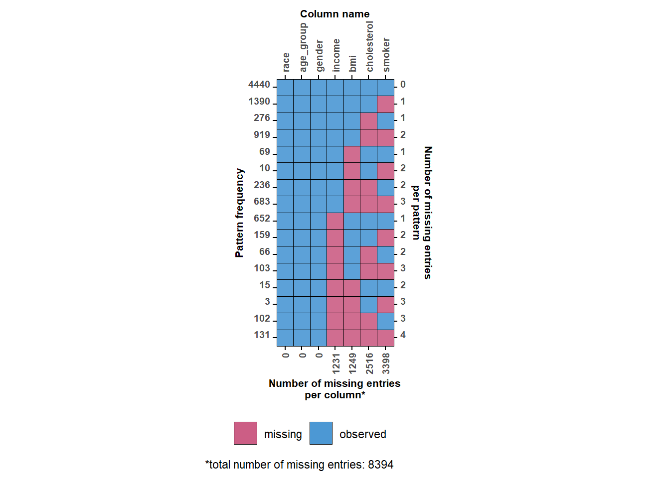
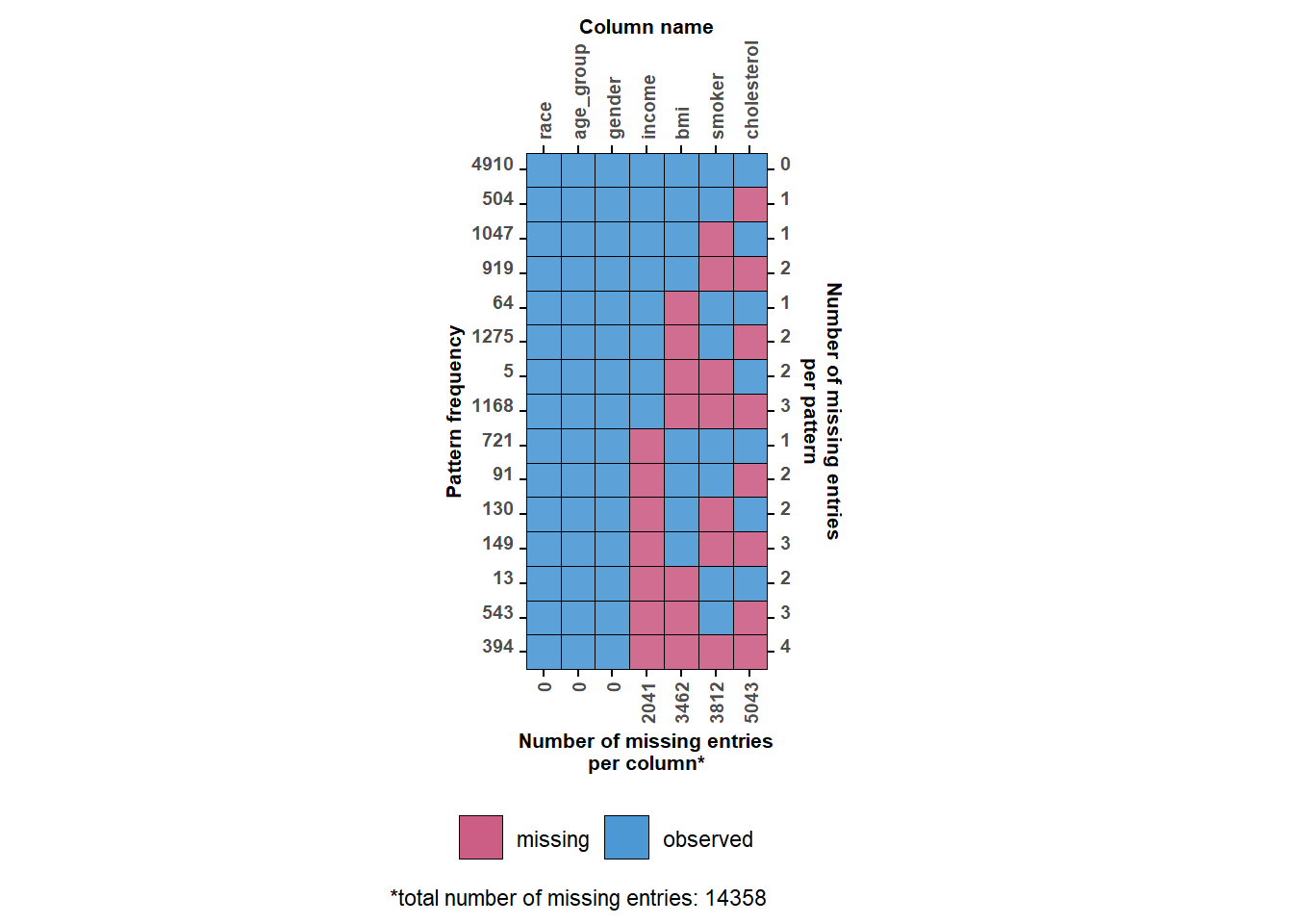
What it showsThe analysis retained 21,187 records: 9,254 Pre-COVID and 11,933 Post-COVID. Four variables contained missing values, with the largest reported rates in smoking status and cholesterol.
Why it mattersComplete-case deletion would discard information unevenly and could change the period composition. Multiple imputation allows the uncertainty from missing values to enter the final estimates.
LimitationThe missingness classifications are assumptions informed by context, not facts identified from the observed data alone. In particular, suspected MNAR income requires sensitivity analysis.
02 · Initial diagnostic
Predictive mean matching over-concentrated two health measures
Observed density curves were compared with the completed-data curves after the first MICE run.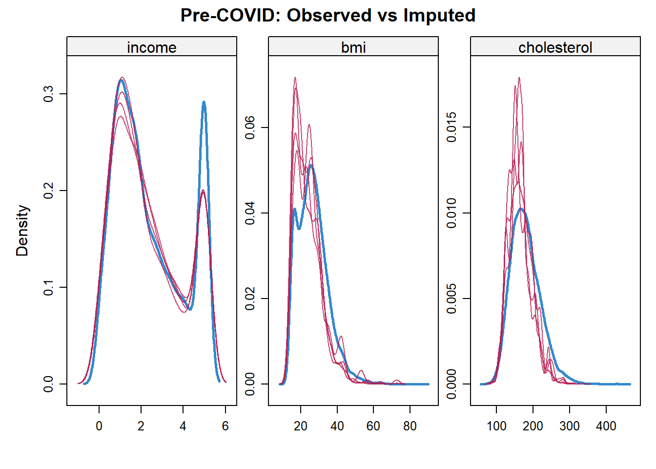
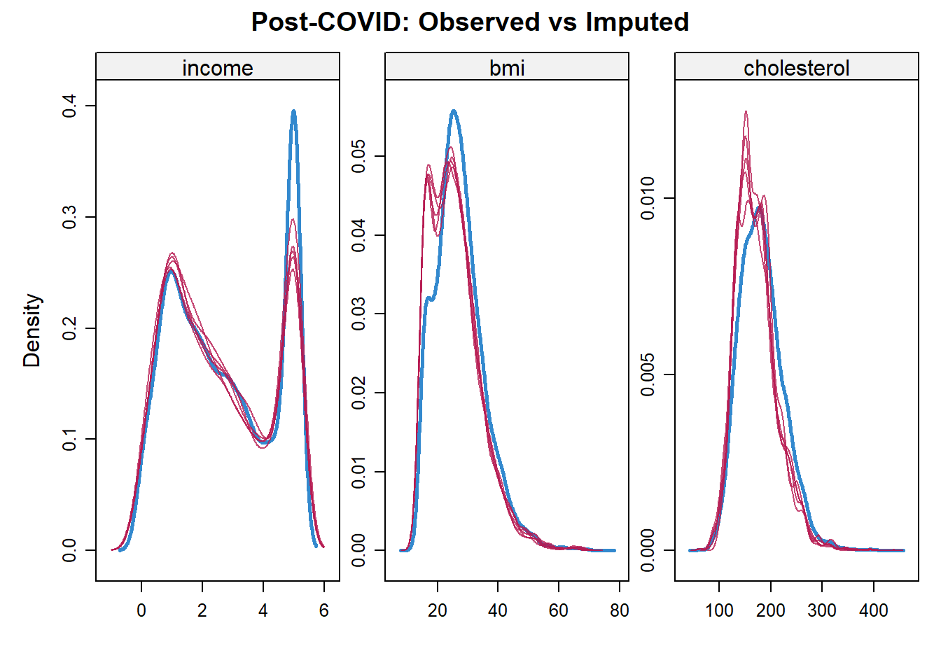
What it showsThe imputed BMI and cholesterol curves were taller and narrower than the corresponding observed curves in both periods. Income was closer in shape, although some differences remained.
Why it mattersAn imputation model that compresses the distribution can understate variability and distort standard errors, interval estimates and relationships with other variables.
LimitationDensity overlays are diagnostic rather than a formal goodness-of-fit test. Close marginal distributions also do not guarantee preservation of multivariable relationships.
03 · Recalibration
Changing the imputation model improved distributional alignment
BMI and cholesterol were switched from PMM to Bayesian linear regression, and the final run used ten completed datasets.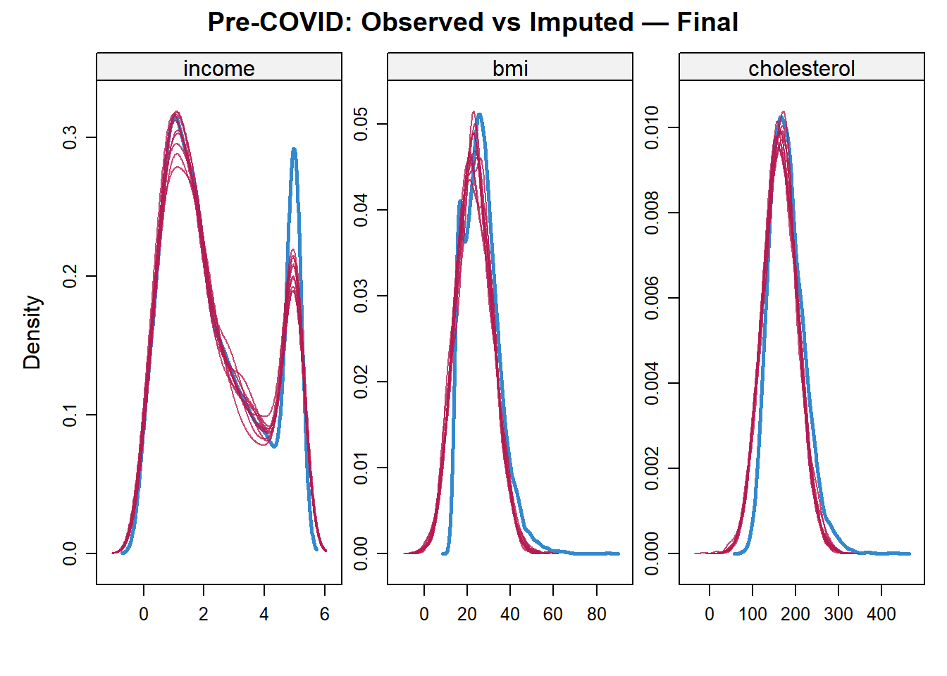
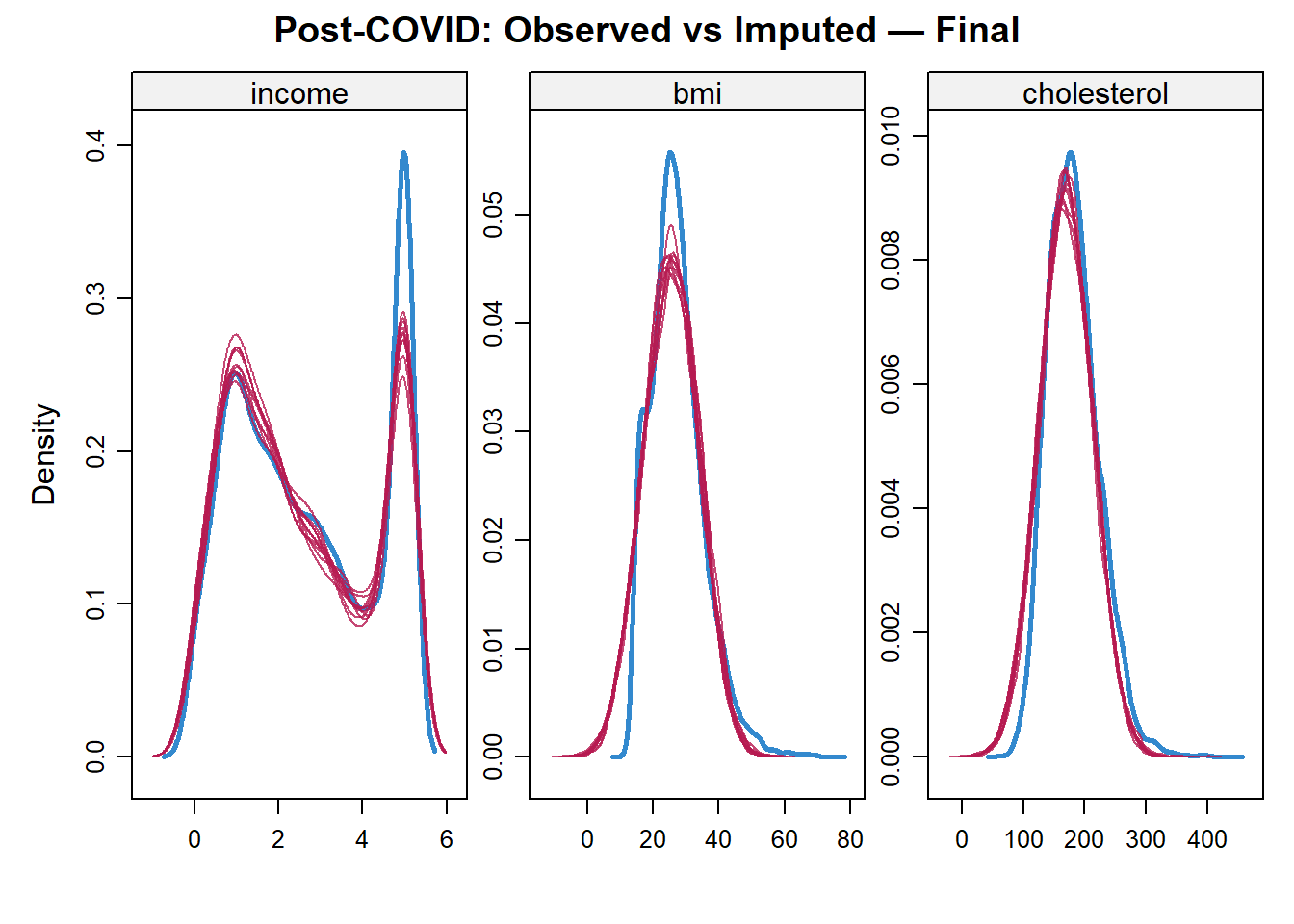
What it showsAfter recalibration, the red imputed BMI and cholesterol curves track the blue observed curves more closely in both periods. The final workflow used 20 iterations and m = 10 imputations.
Why it mattersThe adjustment addresses the visible over-peaking from the initial run and better preserves the continuous spread needed for downstream inference.
LimitationThe normal model can generate implausible values when a variable is bounded or skewed. Range checks, posterior predictive diagnostics and sensitivity runs should accompany the visual improvement.
04 · Pooled period contrasts
BMI remained positive after full pooling; cholesterol did not clear zero
Three interval constructions produced similar centres and different widths, with Rubin's Rules carrying the most complete uncertainty.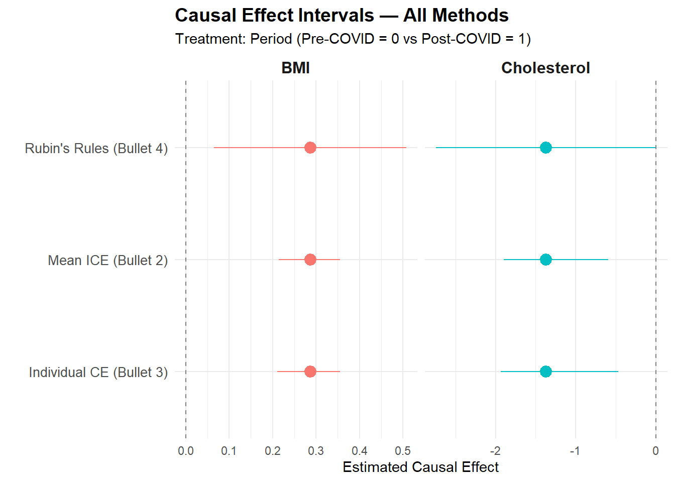
| Outcome | Mean ICE | Individual effect | Rubin's Rules | Inference |
|---|---|---|---|---|
| BMI | 0.21 to 0.36 | ≈ 0.21 to 0.36 | 0.07 to 0.51 | Positive at 5% |
| Cholesterol | −1.90 to −0.60 | ≈ −1.90 to −0.60 | −2.75 to 0.01 | Not significant at 5% |
What it showsThe Rubin-pooled BMI interval was 0.07 to 0.51 and stayed above zero. The cholesterol interval was −2.75 to 0.01 and narrowly crossed zero. Mean-ICE and individual-effect intervals were considerably narrower.
Why it mattersThe formal conclusion changes once within- and between-imputation uncertainty are combined. BMI shows a statistically detectable period difference; cholesterol does not at the 5% threshold.
LimitationThese are Pre-/Post-COVID period contrasts. Calling them causal COVID effects requires additional identification assumptions and control of time-varying confounding that are not established by imputation alone.
05 · Decision framework
The analysis is strongest when the uncertainty is not simplified away
A compact governance view separates what the evidence supports from what still requires sensitivity analysis.| Question | Supported conclusion | Next validation step |
|---|---|---|
| Did recalibration help? | Yes, marginal density alignment improved | Add multivariable and range diagnostics |
| Is BMI different across periods? | Positive pooled interval | Assess design and confounding assumptions |
| Is cholesterol different? | Not at 5% under Rubin pooling | Report effect and uncertainty, not a binary claim alone |
| Is income MNAR resolved? | No | Run delta-adjustment or pattern-mixture sensitivity analysis |
| Is the contrast causal? | Not established by MICE | Defend exchangeability and time-varying confounding control |
What it showsRubin's Rules changes the strength of the cholesterol conclusion, while the suspected MNAR income mechanism and causal identification remain unresolved by the completed-data workflow.
Why it mattersA defensible report must distinguish imputation uncertainty, missingness assumptions and causal assumptions. Solving one layer does not automatically solve the others.
LimitationThe conclusions remain sensitive to the missingness assumptions, imputation specification and period-comparison design.
Missingness and imputation design
Income, BMI, cholesterol and smoking status contain missing values. BMI, cholesterol and adult smoking status are treated as Missing at Random, while income is suspected to be Missing Not at Random. Structural missingness for children aged 0-17 is kept separate from adult smoking nonresponse.
The initial workflow used predictive mean matching for continuous variables and logistic regression for smoking status. Income was excluded as a predictor for other variables. That restriction reduces one route for contamination, although it does not by itself solve an MNAR mechanism.
Why the imputation model changed
Initial density plots showed that predictive mean matching concentrated imputed BMI and cholesterol values too tightly around their central regions. The final workflow therefore retained PMM for income and switched BMI and cholesterol to Bayesian linear regression before increasing the number of completed datasets to ten.
The revised density overlays followed the observed shapes more closely in both periods. This is useful diagnostic evidence, although distributional similarity alone cannot prove that the missing values were recovered without bias.
Pooled period differences
The BMI contrast was positive across all interval methods. Rubin's Rules produced a 95% interval from 0.07 to 0.51, which remained above zero. The cholesterol contrast was negative, while its pooled interval from −2.75 to 0.01 crossed zero and therefore did not meet the conventional 5% significance threshold.
The narrower mean-ICE and individual-effect intervals omit part of the uncertainty captured by formal multiple-imputation pooling. Rubin's Rules is therefore the appropriate result to lead the conclusion.
Interpretation and limitations
The analysis supports a statistically detectable difference in BMI between the observed periods and an inconclusive difference in cholesterol after pooled uncertainty is included. These estimates should be described as adjusted period contrasts unless the causal identification assumptions are established separately.
A causal COVID interpretation would require defensible exchangeability, measurement consistency and control of time-varying confounding. The suspected MNAR income process also requires sensitivity analysis or an explicit non-ignorable model; removing income from the predictor matrix does not make the mechanism ignorable.
- Report Rubin-pooled intervals as the primary inferential result.
- Add sensitivity analysis for the suspected MNAR income mechanism.
- Constrain or review imputed health values for clinical plausibility.
- Treat Pre-/Post-COVID comparisons as causal only after the identification assumptions are defended.