

Central question
Can statistical and machine-learning count models estimate claim frequency, rank policy risk and remain well calibrated on unseen policies?
Project overview
This project models annualised motor-insurance claim frequency as a count outcome. Exposure enters the GLMs through a log offset and the XGBoost model through its base margin, ensuring that policies observed for different lengths of time remain comparable.
The analysis separates data audit, exploratory work, model development, validation-based selection and final test reporting. Severity variables are kept outside the frequency models to prevent target leakage.
358,483 policy-years of exposure
Highly sparse count outcome
26,444 observed claims
Final refit XGBoost
Evidence summary
Sparse claims, calibrated forecasts and a measurable ranking gain
The case study follows the complete modelling path from portfolio audit and GLM evolution to validation-led selection, test calibration, residual checks and explainability.01 · Portfolio audit
More than 96% of policies recorded no claim
The outcome was a sparse count, making exposure-aware count modelling essential.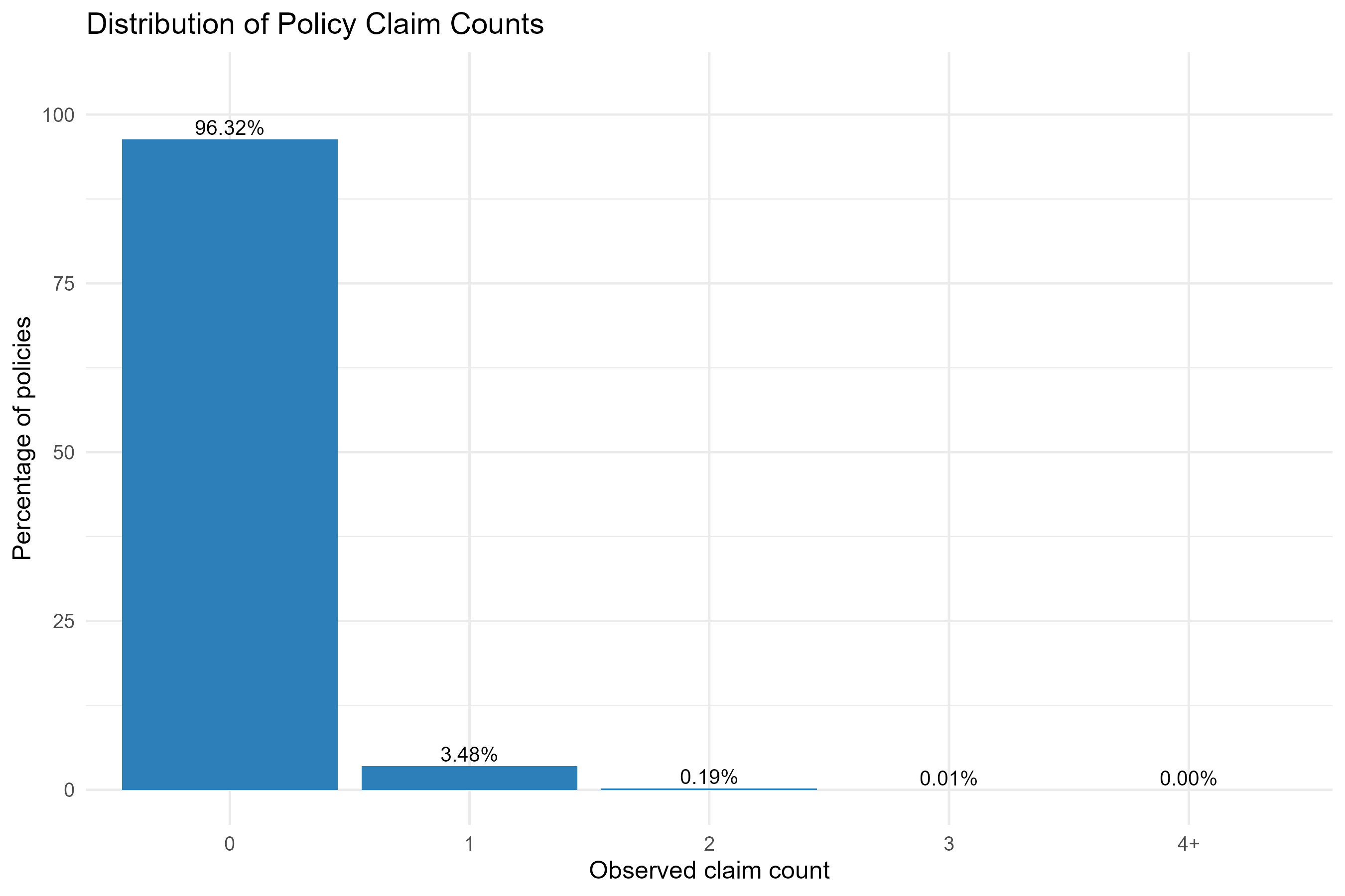
| Sample | Policies | Exposure | Claims | Claim frequency |
|---|---|---|---|---|
| Full portfolio | 677,991 | 358,482.84 | 26,444 | 0.07377 |
| Training | 406,793 | 214,928.97 | 15,868 | 0.07383 |
| Validation | 135,597 | 71,824.16 | 5,292 | 0.07368 |
| Test | 135,601 | 71,729.70 | 5,284 | 0.07367 |
What it showsAcross 677,991 policies and 358,483 policy-years, the portfolio recorded 26,444 claims. Zero claims were observed for 96.32% of policies, one claim for 3.48% and two or more for only 0.20%.
Why it mattersThe distribution rules out ordinary linear regression and explains the use of Poisson-family likelihoods and a Poisson XGBoost objective.
LimitationThe public freMTPL2 portfolio represents one insurance market and period. Model performance and feature relationships may not transfer unchanged to another book of business.
02 · GLM evolution
Exposure and nonlinear terms produced the useful GLM gains
Validation mean Poisson deviance, rather than training fit alone, guided model complexity.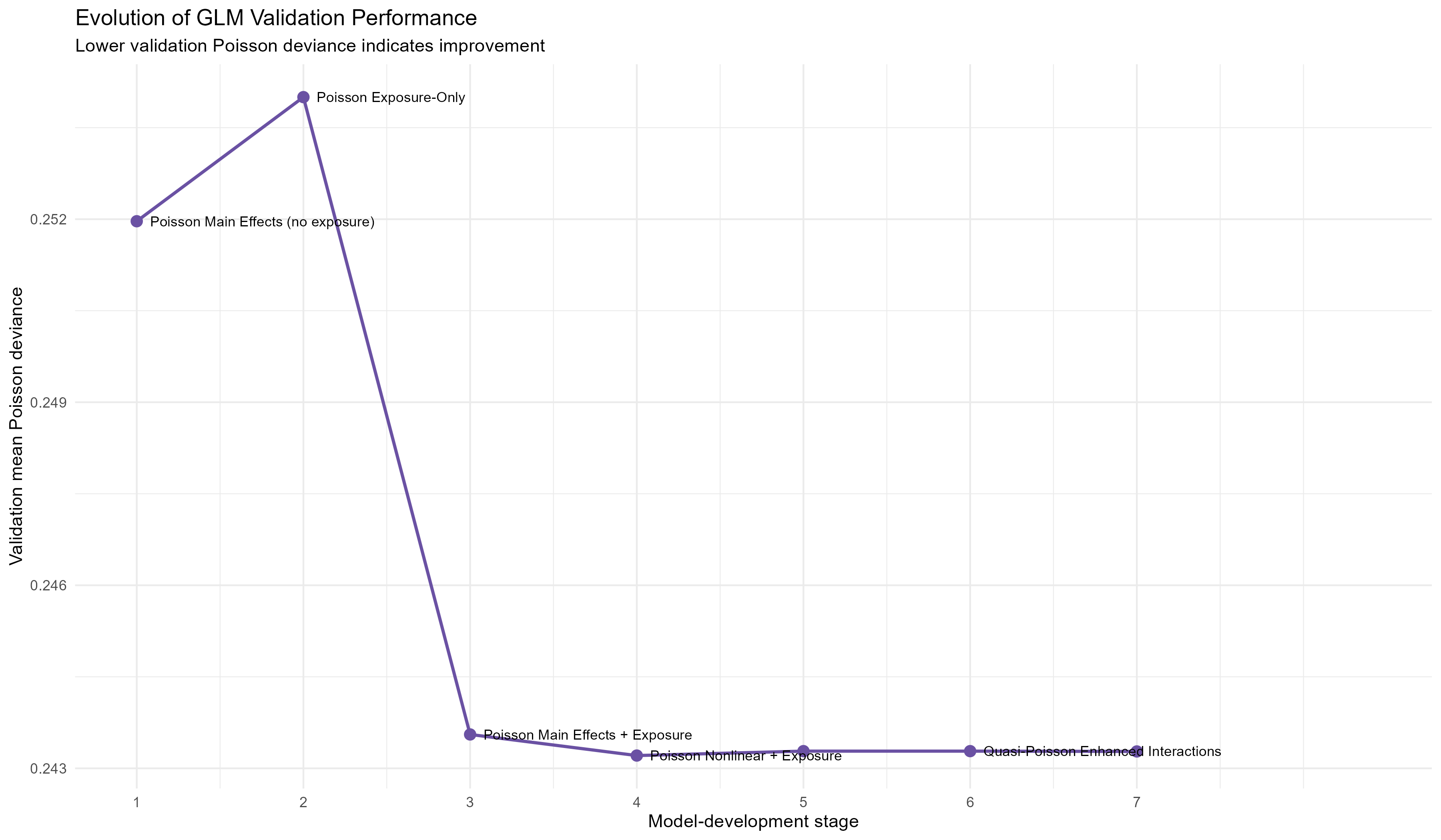
| Model | MAE | RMSE | Poisson deviance | Gini | A/E |
|---|---|---|---|---|---|
| XGBoost Poisson + exposure | 0.07213 | 0.20523 | 0.23634 | 0.34420 | 0.99536 |
| Poisson nonlinear + exposure | 0.07309 | 0.20704 | 0.24321 | 0.28967 | 0.99817 |
| Negative binomial + interactions | 0.07324 | 0.20705 | 0.24328 | 0.28797 | 0.99429 |
What it showsAdding rating factors and the exposure offset reduced validation deviance from about .252-.254 to .244. Nonlinear terms improved it further to .24321, while extra interactions produced no meaningful validation gain.
Why it mattersThe curve identifies where additional complexity stopped improving unseen-policy performance and supports the nonlinear Poisson model as the GLM finalist.
LimitationThe negative-binomial interaction model achieved the best training AIC and BIC, yet its validation deviance was slightly worse. Information criteria and held-out predictive performance answer different questions.
03 · Final test comparison
XGBoost improved risk ranking without losing aggregate calibration
Both finalists were refitted on training plus validation data before the untouched test set was scored.| Model | Predicted claims | A/E | MAE | RMSE | Deviance | Gini |
|---|---|---|---|---|---|---|
| XGBoost Poisson | 5,283.59 | 1.00008 | 0.07200 | 0.20133 | 0.23554 | 0.34456 |
| Nonlinear Poisson GLM | 5,285.75 | 0.99967 | 0.07301 | 0.20278 | 0.24156 | 0.29182 |
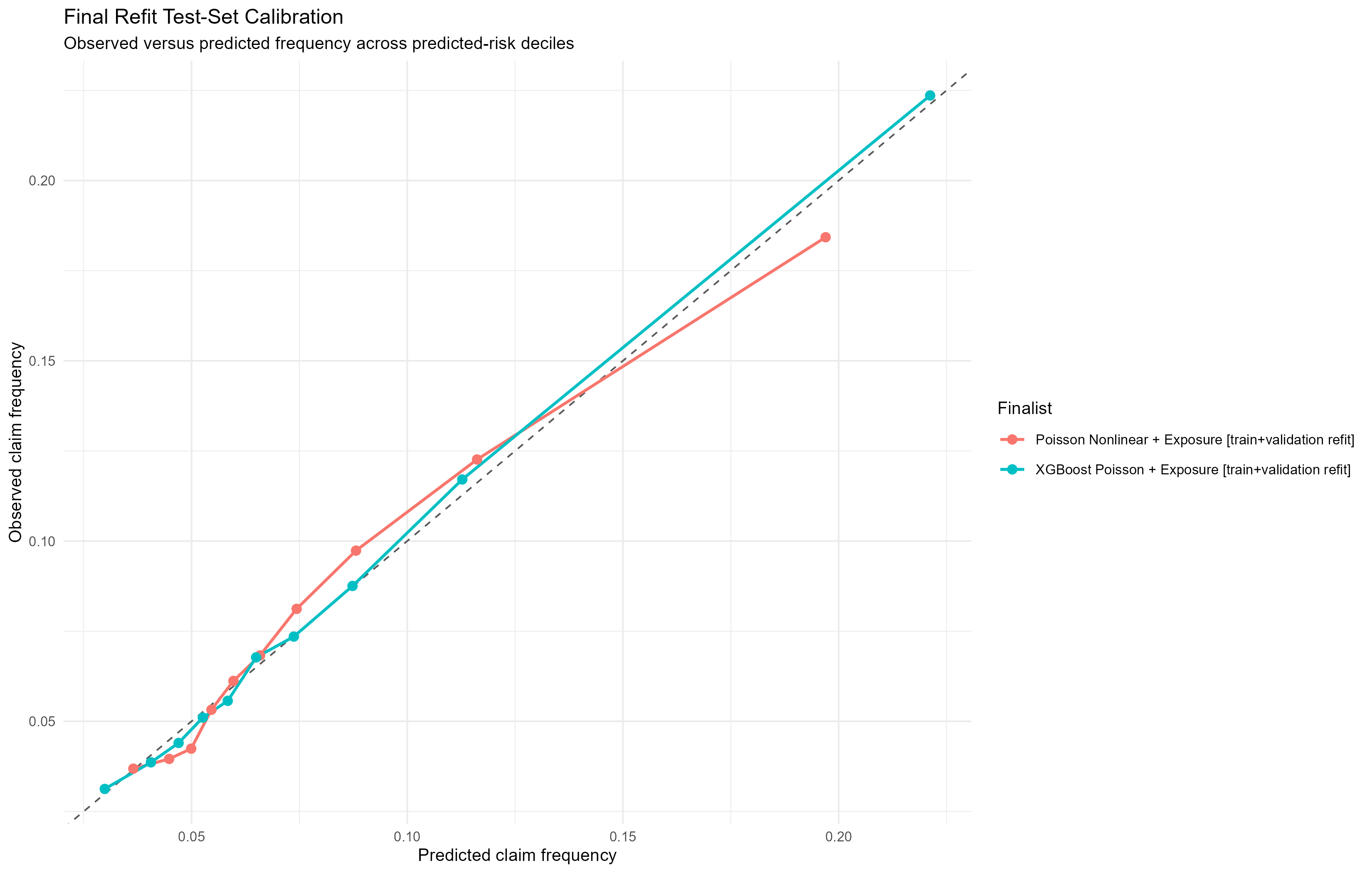
What it showsXGBoost achieved test deviance .23554 and Gini .34456, compared with .24156 and .29182 for the nonlinear Poisson GLM. It predicted 5,283.6 claims against 5,284 observed, giving A/E = 1.00008.
Why it mattersThe machine-learning model produced a clear discrimination gain and retained portfolio-level calibration. Its RMSE advantage was smaller, so the benefit is mainly stronger risk ordering rather than a dramatic reduction in row-level error.
LimitationAggregate A/E can conceal local miscalibration. The decile chart should be monitored on new data, especially in the highest-risk segment where small deviations matter most.
04 · Explainability
Bonus-malus dominated the nonlinear model
Gain-based importance identifies the variables XGBoost used most strongly when splitting the portfolio.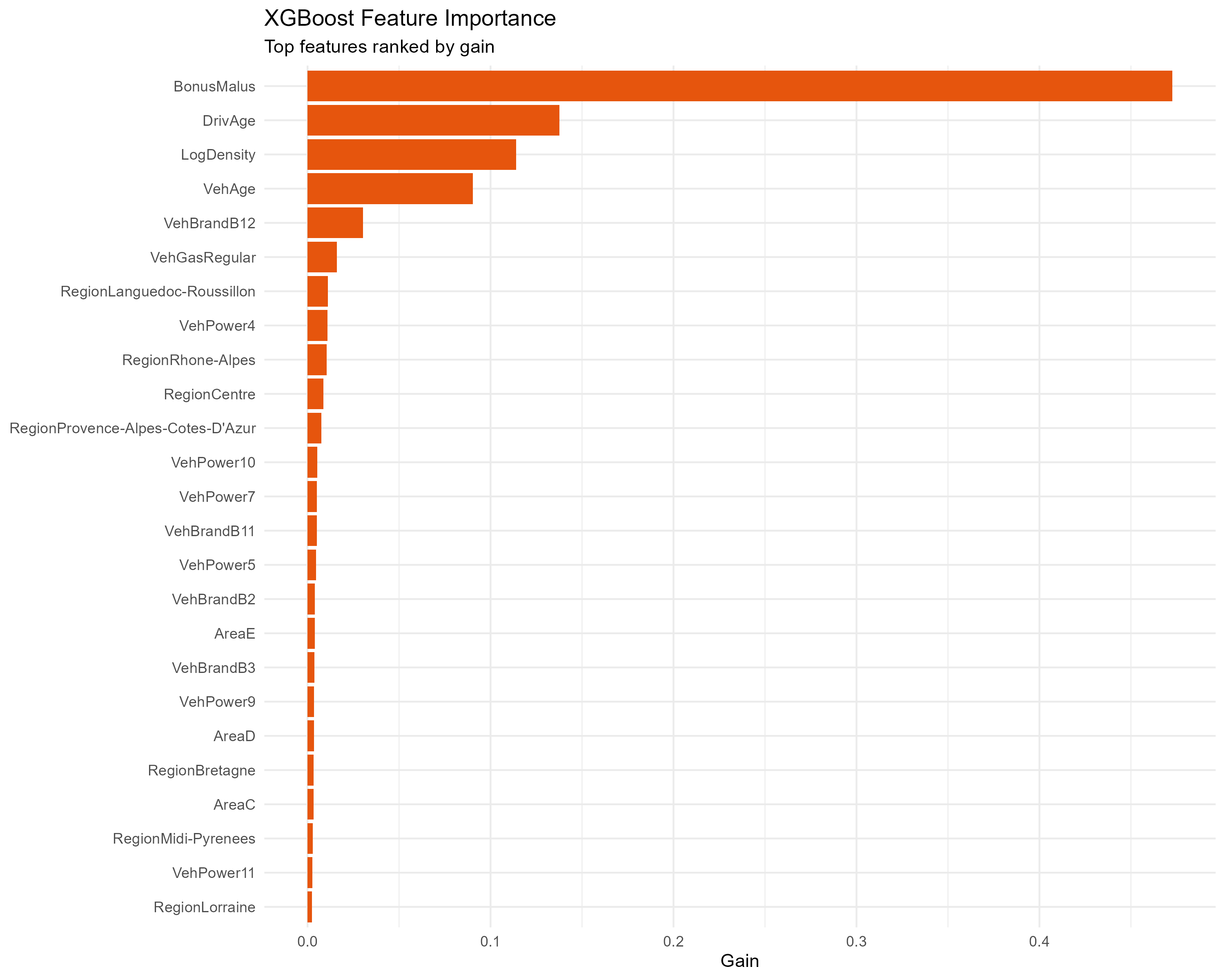
What it showsBonus-malus contributed 47.3% of total split gain, followed by driver age at 13.8%, log density at 11.4% and vehicle age at 9.0%. The remaining individual features were much smaller.
Why it mattersThe ranking highlights the policy and driver characteristics most useful for separating low- and high-frequency risk within this dataset.
LimitationImportance is not an effect direction or a causal estimate. Correlated variables can share or displace importance, and rating factors require governance and fairness review before operational use.
05 · GLM diagnostics
Good calibration did not remove every residual concern
Simulation-based DHARMa checks were run on a representative training sample for the selected nonlinear Poisson GLM.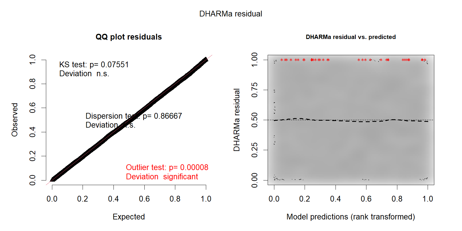
| Test | Statistic | p-value | Decision at 5% |
|---|---|---|---|
| Uniformity | 0.01045 | .0755 | No concern flagged |
| Dispersion | 0.98937 | .8667 | No concern flagged |
| Zero inflation | 1.00322 | .0400 | Concern flagged |
| Outliers | 256 | < .001 | Concern flagged |
What it showsUniformity (p = .076) and dispersion (p = .867) were not flagged at 5%. Zero inflation (p = .040) and outliers (p < .001) remained significant.
Why it mattersThe selected GLM is a useful transparent benchmark, yet its distributional assumptions do not fully reproduce rare or excess-zero behaviour in the data.
LimitationDHARMa was run on a representative sample for computational feasibility. Diagnostic significance should be combined with effect size, plots and out-of-sample behaviour rather than used as an automatic rejection rule.
Portfolio structure and modelling challenge
The audited portfolio contained 677,991 unique policies, 358,483 policy-years of exposure and 26,444 claims. Most policies recorded no claim, 3.48% recorded one claim and only 0.20% recorded two or more.
That sparsity makes ordinary linear regression unsuitable. The project compared exposure-aware Poisson specifications, quasi-Poisson and negative-binomial alternatives, then introduced XGBoost with a Poisson objective as a nonlinear comparator.
Validation-led model selection
The nonlinear Poisson GLM was the best GLM on validation mean Poisson deviance. The negative-binomial interaction model achieved the lowest in-sample AIC and BIC, yet it did not generalise as well on the validation criterion. This distinction prevented an in-sample fit statistic from deciding the final model.
XGBoost ranked first on validation data and was therefore refitted on the combined training and validation sample before the untouched test set was evaluated.
Final test result
On 135,601 test policies, final-refit XGBoost predicted 5,283.6 claims against 5,284 observed, giving an actual-to-expected ratio of 1.00008. It achieved MAE 0.0720, RMSE 0.2013, mean Poisson deviance 0.2355 and normalised Gini 0.3446.
The final nonlinear Poisson GLM was also well calibrated at portfolio level, with an actual-to-expected ratio of 0.99967. Its test deviance was 0.2416 and Gini was 0.2918. XGBoost therefore added more ranking power while preserving aggregate calibration, although its raw-error advantage was modest.
Diagnostics, interpretation and governance
DHARMa checks for the selected GLM found no uniformity or dispersion concern at the 5% level, while zero-inflation and outlier tests remained significant. This means good portfolio-level calibration does not remove all distributional misspecification.
Bonus-malus score was the strongest XGBoost feature, followed by driver age, log population density and vehicle age. These rankings describe predictive contribution rather than causal effects and should be monitored for stability and fairness before operational pricing use.
People behind the project